CohortCharacteristics

A R package to Characterise cohorts

CohortCharacteristics

Website

Cohort characteristics is on cran:

install.packages("CohortCharacteristics")

You can also install the development version from our github repo:

remotes::install_github("darwin-eu/CohortCharacteristics")

The documentation and vignettes of the packages can be found in our page: https://darwin-eu.github.io/CohortCharacteristics/

Let’s get started

library(CohortCharacteristics)
library(omock)
library(CohortConstructor)
library(visOmopResults)
library(dplyr)
library(PatientProfiles)
library(plotly)

Let’s get started

First we will create a cdm_reference from GiBleed database:

cdm <- mockCdmFromDataset(datasetName = "GiBleed", source = "duckdb")

cdm

── # OMOP CDM reference (duckdb) of GiBleed ────────────────────────────────────────────────────────────────────────────

• omop tables: care_site, cdm_source, concept, concept_ancestor, concept_class, concept_relationship, concept_synonym,
condition_era, condition_occurrence, cost, death, device_exposure, domain, dose_era, drug_era, drug_exposure,
drug_strength, fact_relationship, location, measurement, metadata, note, note_nlp, observation, observation_period,
payer_plan_period, person, procedure_occurrence, provider, relationship, source_to_concept_map, specimen, visit_detail,
visit_occurrence, vocabulary

• cohort tables: -

• achilles tables: -

• other tables: -

Workflow

We have three types of functions:

summarise: these functions produce an standardised output to summarise a cohort. This standard output is called summarised_result.
plot: these functions produce plots (currently, only ggplot, but working to implement plotly) from a summarised_result object.
table: these functions produce tables (gt and flextable) from a summarised_result object.

Set the style

setGlobalTableOptions(style = "darwin")
setGlobalPlotOptions(style = "darwin")

Summarise cohort entries

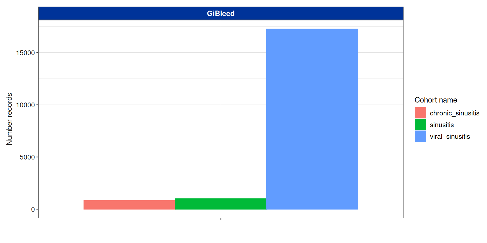
We can start instantiating a cohort:

cdm$my_cohort <- conceptCohort(
  cdm = cdm,
  conceptSet = list(
    viral_sinusitis = 40481087L,
    sinusitis = 4283893L,
    chronic_sinusitis = 257012L
  ),
  name = "my_cohort"
)
cohortCount(cdm$my_cohort)

# A tibble: 3 × 3
  cohort_definition_id number_records number_subjects
                 <int>          <int>           <int>
1                    1            825             812
2                    2           1001             833
3                    3          17268            2686

Summarise cohort entries

result <- summariseCohortCount(cdm$my_cohort)

tableCohortCount(result = result)

CDM name	Variable name	Estimate name	Cohort name
CDM name	Variable name	Estimate name	chronic_sinusitis	sinusitis	viral_sinusitis
GiBleed	Number records	N	825	1,001	17,268
	Number subjects	N	812	833	2,686

Summarise cohort entries

result |>
  filter(variable_name == "Number records") |>
  plotCohortCount(colour = "cohort_name")

Summarise cohort entries

Now we can apply some inclusion criteria:

cdm$my_cohort <- cdm$my_cohort |>
  requireAge(ageRange = c(0, 15))
cohortCount(cdm$my_cohort)

# A tibble: 3 × 3
  cohort_definition_id number_records number_subjects
                 <int>          <int>           <int>
1                    1            260             260
2                    2            278             265
3                    3           4624            2223

cdm$my_cohort <- cdm$my_cohort |>
  requirePriorObservation(minPriorObservation = 365)
cohortCount(cdm$my_cohort)

# A tibble: 3 × 3
  cohort_definition_id number_records number_subjects
                 <int>          <int>           <int>
1                    1            243             243
2                    2            260             249
3                    3           4360            2168

Summarise cohort entries

This data has been stored in the attrition attribute

attrition(cdm$my_cohort) |>
  glimpse()

Rows: 18
Columns: 7
$ cohort_definition_id <int> 1, 1, 1, 1, 1, 1, 2, 2, 2, 2, 2, 2, 3, 3, 3, 3, 3, 3
$ number_records       <int> 825, 825, 825, 825, 260, 243, 1001, 1001, 1001, 1001, 278, 260, 17268, 17268, 17268, 1726…
$ number_subjects      <int> 812, 812, 812, 812, 260, 243, 833, 833, 833, 833, 265, 249, 2686, 2686, 2686, 2686, 2223,…
$ reason_id            <int> 1, 2, 3, 4, 5, 6, 1, 2, 3, 4, 5, 6, 1, 2, 3, 4, 5, 6
$ reason               <chr> "Initial qualifying events", "Record in observation", "Not missing record date", "Merge o…
$ excluded_records     <int> 0, 0, 0, 0, 565, 17, 0, 0, 0, 0, 723, 18, 0, 0, 0, 0, 12644, 264
$ excluded_subjects    <int> 0, 0, 0, 0, 552, 17, 0, 0, 0, 0, 568, 16, 0, 0, 0, 0, 463, 55

Summarise cohort entries

result <- summariseCohortAttrition(cohort = cdm$my_cohort)

tableCohortAttrition(result = result)

Reason	Variable name
Reason	number_records	number_subjects	excluded_records	excluded_subjects
GiBleed; chronic_sinusitis
Initial qualifying events	825	812	0	0
Record in observation	825	812	0	0
Not missing record date	825	812	0	0
Merge overlapping records	825	812	0	0
Age requirement: 0 to 15	260	260	565	552
Prior observation requirement: 365 days	243	243	17	17
GiBleed; sinusitis
Initial qualifying events	1,001	833	0	0
Record in observation	1,001	833	0	0
Not missing record date	1,001	833	0	0
Merge overlapping records	1,001	833	0	0
Age requirement: 0 to 15	278	265	723	568
Prior observation requirement: 365 days	260	249	18	16
GiBleed; viral_sinusitis
Initial qualifying events	17,268	2,686	0	0
Record in observation	17,268	2,686	0	0
Not missing record date	17,268	2,686	0	0
Merge overlapping records	17,268	2,686	0	0
Age requirement: 0 to 15	4,624	2,223	12,644	463
Prior observation requirement: 365 days	4,360	2,168	264	55

Summarise cohort entries

plotCohortAttrition(result = result, type = "png")

Summarise cohort overlap

It can be useful to identify the individuals that are in two cohorts:

result <- summariseCohortOverlap(cohort = cdm$my_cohort)

tableCohortOverlap(result)

Cohort name reference	Cohort name comparator	Estimate name	Variable name
Cohort name reference	Cohort name comparator	Estimate name	Only in reference cohort	In both cohorts	Only in comparator cohort
GiBleed
chronic_sinusitis	sinusitis	N (%)	103 (29.26%)	140 (39.77%)	109 (30.97%)
	viral_sinusitis	N (%)	51 (2.30%)	192 (8.65%)	1,976 (89.05%)
sinusitis	viral_sinusitis	N (%)	52 (2.34%)	197 (8.87%)	1,971 (88.78%)

Summarise cohort overlap

plotCohortOverlap(result = result)

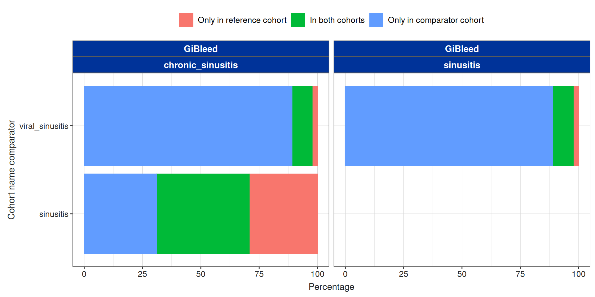
Summarise cohort overlap

By default the overlap is done at the subject_id level, but we can customise this and use more columns:

result <- summariseCohortOverlap(cohort = cdm$my_cohort, overlapBy = c("subject_id", "cohort_start_date"))

tableCohortOverlap(result = result)

Cohort name reference	Cohort name comparator	Estimate name	Variable name
Cohort name reference	Cohort name comparator	Estimate name	Only in reference cohort	In both cohorts	Only in comparator cohort
GiBleed
chronic_sinusitis	sinusitis	N (%)	243 (48.31%)	0 (0.00%)	260 (51.69%)
	viral_sinusitis	N (%)	243 (5.28%)	0 (0.00%)	4,360 (94.72%)
sinusitis	viral_sinusitis	N (%)	260 (5.63%)	0 (0.00%)	4,360 (94.37%)

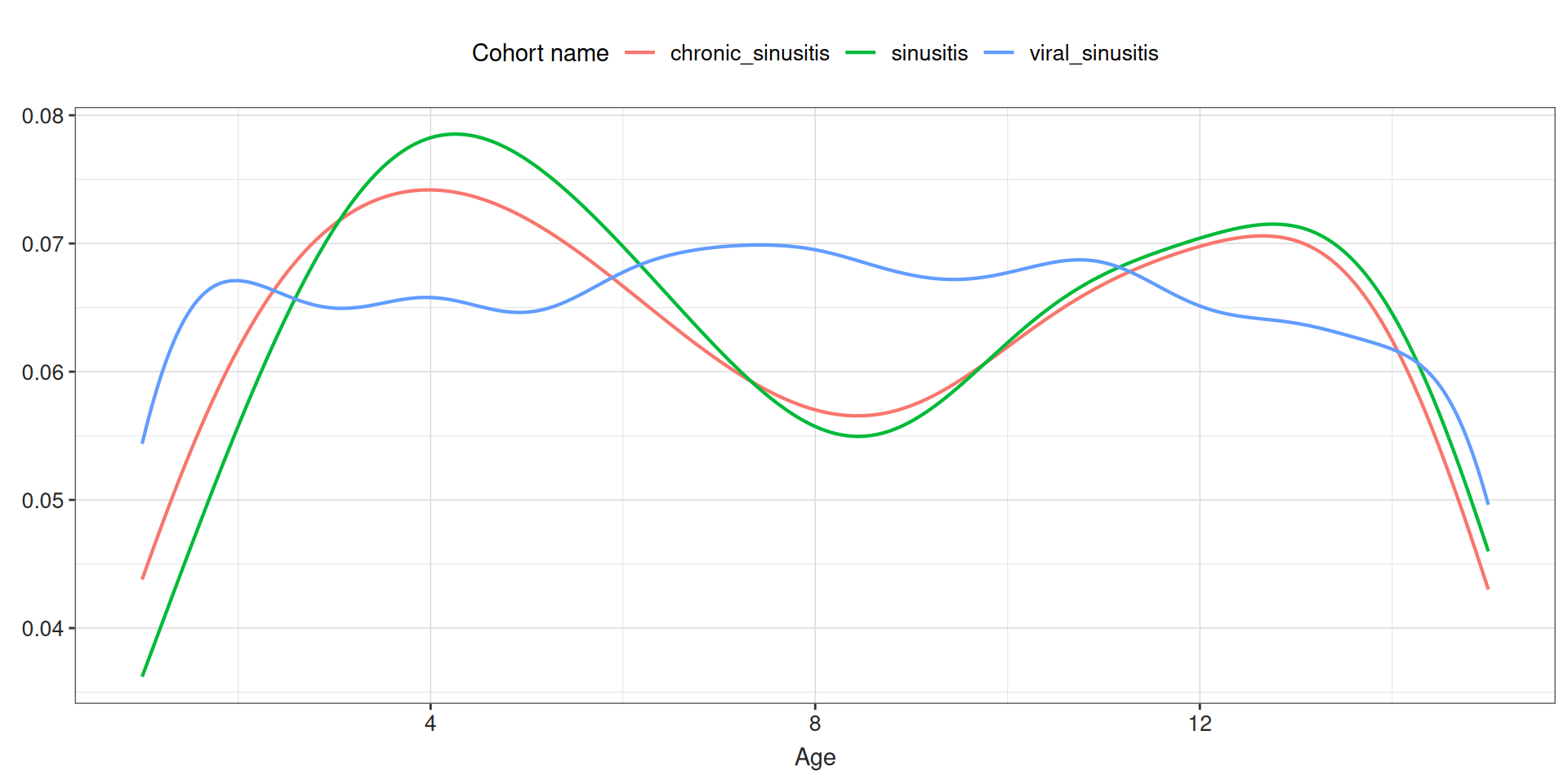
Summarise cohort characteristics

To get summary of the characteristics for your cohort you can use summariseCharacteristics():

result <- summariseCharacteristics(cohort = cdm$my_cohort)

Summarise cohort characteristics

tableCharacteristics(result = result, header = "cohort_name")

CDM name	Variable name	Variable level	Estimate name	Cohort name
CDM name	Variable name	Variable level	Estimate name	chronic_sinusitis	sinusitis	viral_sinusitis
GiBleed	Number records	–	N	243	260	4,360
	Number subjects	–	N	243	249	2,168
	Cohort start date	–	Median [Q25 - Q75]	1969-04-01 [1957-12-24 - 1980-08-02]	1970-10-06 [1957-09-05 - 1981-07-24]	1969-04-22 [1957-12-03 - 1979-05-19]
			Range	1911-12-12 to 1998-09-29	1911-10-31 to 1998-09-01	1910-10-21 to 1999-11-02
	Cohort end date	–	Median [Q25 - Q75]	1969-10-19 [1958-09-07 - 1981-06-23]	1971-01-08 [1957-10-31 - 1981-10-30]	1969-05-08 [1957-12-15 - 1979-06-01]
			Range	1911-12-12 to 2011-09-26	1912-01-23 to 1998-10-13	1910-11-04 to 1999-11-23
	Age	–	Median [Q25 - Q75]	8 [4 - 12]	8 [4 - 12]	8 [4 - 12]
			Mean (SD)	7.92 (4.37)	8.10 (4.32)	7.92 (4.30)
			Range	1 to 15	1 to 15	1 to 15
	Sex	Female	N (%)	124 (51.03%)	142 (54.62%)	2,206 (50.60%)
		Male	N (%)	119 (48.97%)	118 (45.38%)	2,154 (49.40%)
	Prior observation	–	Median [Q25 - Q75]	3,052 [1,657 - 4,528]	3,118 [1,795 - 4,487]	3,068 [1,714 - 4,407]
			Mean (SD)	3,079.56 (1,600.95)	3,142.19 (1,562.49)	3,076.48 (1,574.41)
			Range	388 to 5,832	398 to 5,815	365 to 5,842
	Future observation	–	Median [Q25 - Q75]	17,643 [13,899 - 22,168]	17,557 [13,719 - 22,300]	17,884 [14,241 - 21,779]
			Mean (SD)	18,330.67 (5,753.00)	18,518.75 (6,356.40)	18,457.77 (5,674.75)
			Range	6,986 to 39,045	7,014 to 39,087	6,530 to 39,020
	Days in cohort	–	Median [Q25 - Q75]	1 [1 - 1]	57 [36 - 102]	15 [8 - 22]
			Mean (SD)	317.64 (1,762.31)	79.59 (62.56)	15.02 (5.68)
			Range	1 to 13,234	15 to 428	7 to 23
	Days to next record	–	Median [Q25 - Q75]	–	1,266 [854 - 2,302]	1,115 [488 - 1,957]
			Mean (SD)	–	1,679.00 (1,078.99)	1,353.50 (1,058.41)
			Range	–	636 to 4,072	35 to 5,227

Summarise cohort characteristics

By default we have seen how demographics are characterised, by we can do more.

result <- summariseCharacteristics(
  cohort = cdm$my_cohort,
  ageGroup = list(c(0, 4), c(5, 9), c(10, 14), c(15, Inf))
)

tableCharacteristics(result = result)

			CDM name
			GiBleed
Variable name	Variable level	Estimate name	Cohort name
Variable name	Variable level	Estimate name	chronic_sinusitis	sinusitis	viral_sinusitis
Number records	–	N	243	260	4,360
Number subjects	–	N	243	249	2,168
Cohort start date	–	Median [Q25 - Q75]	1969-04-01 [1957-12-24 - 1980-08-02]	1970-10-06 [1957-09-05 - 1981-07-24]	1969-04-22 [1957-12-03 - 1979-05-19]
		Range	1911-12-12 to 1998-09-29	1911-10-31 to 1998-09-01	1910-10-21 to 1999-11-02
Cohort end date	–	Median [Q25 - Q75]	1969-10-19 [1958-09-07 - 1981-06-23]	1971-01-08 [1957-10-31 - 1981-10-30]	1969-05-08 [1957-12-15 - 1979-06-01]
		Range	1911-12-12 to 2011-09-26	1912-01-23 to 1998-10-13	1910-11-04 to 1999-11-23
Age	–	Median [Q25 - Q75]	8 [4 - 12]	8 [4 - 12]	8 [4 - 12]
		Mean (SD)	7.92 (4.37)	8.10 (4.32)	7.92 (4.30)
		Range	1 to 15	1 to 15	1 to 15
Age group	0 to 4	N (%)	70 (28.81%)	70 (26.92%)	1,180 (27.06%)
	5 to 9	N (%)	72 (29.63%)	78 (30.00%)	1,471 (33.74%)
	10 to 14	N (%)	90 (37.04%)	96 (36.92%)	1,424 (32.66%)
	15 or above	N (%)	11 (4.53%)	16 (6.15%)	285 (6.54%)
Sex	Female	N (%)	124 (51.03%)	142 (54.62%)	2,206 (50.60%)
	Male	N (%)	119 (48.97%)	118 (45.38%)	2,154 (49.40%)
Prior observation	–	Median [Q25 - Q75]	3,052 [1,657 - 4,528]	3,118 [1,795 - 4,487]	3,068 [1,714 - 4,407]
		Mean (SD)	3,079.56 (1,600.95)	3,142.19 (1,562.49)	3,076.48 (1,574.41)
		Range	388 to 5,832	398 to 5,815	365 to 5,842
Future observation	–	Median [Q25 - Q75]	17,643 [13,899 - 22,168]	17,557 [13,719 - 22,300]	17,884 [14,241 - 21,779]
		Mean (SD)	18,330.67 (5,753.00)	18,518.75 (6,356.40)	18,457.77 (5,674.75)
		Range	6,986 to 39,045	7,014 to 39,087	6,530 to 39,020
Days in cohort	–	Median [Q25 - Q75]	1 [1 - 1]	57 [36 - 102]	15 [8 - 22]
		Mean (SD)	317.64 (1,762.31)	79.59 (62.56)	15.02 (5.68)
		Range	1 to 13,234	15 to 428	7 to 23
Days to next record	–	Median [Q25 - Q75]	–	1,266 [854 - 2,302]	1,115 [488 - 1,957]
		Mean (SD)	–	1,679.00 (1,078.99)	1,353.50 (1,058.41)
		Range	–	636 to 4,072	35 to 5,227

Summarise cohort characteristics

We can stratify the characterisation using columns, for example we will characterise the cohort sinusitis by sex.

result <- cdm$my_cohort |>
  addSex() |>
  summariseCharacteristics(
    cohortId = "sinusitis",
    strata = "sex",
    ageGroup = list(c(0, 4), c(5, 9), c(10, 14), c(15, Inf))
  )

tableCharacteristics(result = result, header = "sex", hide = c("cdm_name", "cohort_name", "table_name"))

Variable name	Variable level	Estimate name	Sex
Variable name	Variable level	Estimate name	overall	Female	Male
Number records	–	N	260	142	118
Number subjects	–	N	249	136	113
Cohort start date	–	Median [Q25 - Q75]	1970-10-06 [1957-09-05 - 1981-07-24]	1968-07-14 [1957-08-19 - 1981-01-18]	1972-09-21 [1958-01-04 - 1982-02-27]
		Range	1911-10-31 to 1998-09-01	1912-12-29 to 1998-09-01	1911-10-31 to 1997-05-28
Cohort end date	–	Median [Q25 - Q75]	1971-01-08 [1957-10-31 - 1981-10-30]	1968-08-30 [1957-10-14 - 1981-03-30]	1973-02-16 [1958-02-21 - 1982-07-11]
		Range	1912-01-23 to 1998-10-13	1913-08-31 to 1998-10-13	1912-01-23 to 1997-07-02
Age	–	Median [Q25 - Q75]	8 [4 - 12]	7 [4 - 11]	9 [5 - 12]
		Mean (SD)	8.10 (4.32)	7.63 (4.43)	8.68 (4.12)
		Range	1 to 15	1 to 15	1 to 15
Age group	0 to 4	N (%)	70 (26.92%)	46 (32.39%)	24 (20.34%)
	5 to 9	N (%)	78 (30.00%)	41 (28.87%)	37 (31.36%)
	10 to 14	N (%)	96 (36.92%)	45 (31.69%)	51 (43.22%)
	15 or above	N (%)	16 (6.15%)	10 (7.04%)	6 (5.08%)
Sex	Female	N (%)	142 (54.62%)	142 (100.00%)	–
	Male	N (%)	118 (45.38%)	–	118 (100.00%)
Prior observation	–	Median [Q25 - Q75]	3,118 [1,795 - 4,487]	2,716 [1,605 - 4,279]	3,402 [2,032 - 4,602]
		Mean (SD)	3,142.19 (1,562.49)	2,975.84 (1,598.37)	3,342.37 (1,500.52)
		Range	398 to 5,815	398 to 5,815	517 to 5,766
Future observation	–	Median [Q25 - Q75]	17,557 [13,719 - 22,300]	18,181 [13,841 - 22,321]	16,902 [13,182 - 22,228]
		Mean (SD)	18,518.75 (6,356.40)	18,904.92 (6,314.96)	18,054.03 (6,401.80)
		Range	7,014 to 39,087	7,014 to 38,795	7,777 to 39,087
Days in cohort	–	Median [Q25 - Q75]	57 [36 - 102]	57 [36 - 92]	64 [36 - 120]
		Mean (SD)	79.59 (62.56)	73.57 (56.46)	86.84 (68.73)
		Range	15 to 428	15 to 323	15 to 428
Days to next record	–	Median [Q25 - Q75]	1,266 [854 - 2,302]	1,396 [810 - 1,878]	1,266 [920 - 2,692]
		Mean (SD)	1,679.00 (1,078.99)	1,455.17 (780.82)	1,947.60 (1,408.23)
		Range	636 to 4,072	636 to 2,648	788 to 4,072

Summarise cohort characteristics

We can also summarise the prior conditions. We will need either a codelist of conditions or a prior instantiated cohort. In this case we will create a cohort:

cdm$conditions <- conceptCohort(
  cdm = cdm,
  conceptSet = list(
    hypertension = 4112343L,
    diabetes = 260139L,
    cardiovascular_disease = 372328L
  ),
  name = "conditions"
)

From now on we will use the arguments demographics = FALSE and counts = FALSE to only focus on the part of the characterisation of interest.

Summarise cohort characteristics

result <- cdm$my_cohort |>
  summariseCharacteristics(
    demographics = FALSE, counts = FALSE,
    cohortIntersectFlag = list(
      "Conditions any time prior" = list(
        targetCohortTable = "conditions",
        window = c(-Inf, -1)
      )
    )
  )

tableCharacteristics(result = result)

			CDM name
			GiBleed
Variable name	Variable level	Estimate name	Cohort name
Variable name	Variable level	Estimate name	chronic_sinusitis	sinusitis	viral_sinusitis
Conditions any time prior	Diabetes	N (%)	90 (37.04%)	104 (40.00%)	1,560 (35.78%)
	Cardiovascular disease	N (%)	148 (60.91%)	171 (65.77%)	2,746 (62.98%)
	Hypertension	N (%)	94 (38.68%)	110 (42.31%)	1,910 (43.81%)

Summarise cohort characteristics

Now we will add the number of visit in the prior year:

result <- cdm$my_cohort |>
  summariseCharacteristics(
    demographics = FALSE, counts = FALSE,
    tableIntersectCount = list(
      "Visits in the prior year" = list(
        tableName = "visit_occurrence",
        window = c(-365, -1)
      )
    )
  )

tableCharacteristics(result = result)

			CDM name
			GiBleed
Variable name	Variable level	Estimate name	Cohort name
Variable name	Variable level	Estimate name	chronic_sinusitis	sinusitis	viral_sinusitis
Visits in the prior year	–	Median [Q25 - Q75]	0.00 [0.00 - 0.00]	0.00 [0.00 - 0.00]	0.00 [0.00 - 0.00]
		Mean (SD)	0.00 (0.06)	0.00 (0.06)	0.00 (0.05)
		Range	0.00 to 1.00	0.00 to 1.00	0.00 to 1.00

Summarise cohort characteristics

We could also include time to a prior vaccination, in this case we will define vaccination using a conceptSet:

result <- cdm$my_cohort |>
  summariseCharacteristics(
    demographics = FALSE, counts = FALSE,
    conceptIntersectDays = list(
      "Time to prior vaccines" = list(
        conceptSet = list(vaccine1 = 1127433L, vaccine2 = 40213160L),
        window = c(-Inf, -1),
        order = "last"
      )
    )
  )

tableCharacteristics(result = result)

			CDM name
			GiBleed
Variable name	Variable level	Estimate name	Cohort name
Variable name	Variable level	Estimate name	chronic_sinusitis	sinusitis	viral_sinusitis
Time to prior vaccines	Vaccine2	Median [Q25 - Q75]	-1,399.00 [-2,740.50 - -707.25]	-1,572.00 [-2,762.00 - -710.75]	-1,426.50 [-2,610.00 - -722.25]
		Mean (SD)	-1,710.87 (1,164.27)	-1,769.52 (1,197.58)	-1,695.03 (1,149.73)
		Range	-4,023.00 to -18.00	-4,009.00 to -1.00	-4,239.00 to -1.00
	Vaccine1	Median [Q25 - Q75]	-1,372.00 [-2,048.75 - -600.00]	-1,520.00 [-2,156.50 - -765.00]	-1,291.00 [-2,404.00 - -583.00]
		Mean (SD)	-1,512.57 (1,078.75)	-1,681.07 (1,206.77)	-1,607.13 (1,270.50)
		Range	-5,501.00 to -91.00	-5,438.00 to -78.00	-5,457.00 to -5.00

Summarise cohort characteristics

We have seen that by default the estimates that are calculated are:

count and percentage for binary and categorical variables.
min, q25, median, q75, max, mean and sd for numeric, integer and date variables.

But this can be changed using the estimates argument.

Summarise cohort characteristics

result <- cdm$my_cohort |>
  summariseCharacteristics(
    demographics = FALSE, counts = FALSE,
    conceptIntersectDays = list(
      "Time to prior vaccines" = list(
        conceptSet = list(vaccine1 = 1127433L, vaccine2 = 40213160L),
        window = c(-Inf, -1),
        order = "last"
      )
    ),
    estimates = list(concept_intersect_days = c("q25", "median", "q75"))
  )

tableCharacteristics(result = result)

			CDM name
			GiBleed
Variable name	Variable level	Estimate name	Cohort name
Variable name	Variable level	Estimate name	chronic_sinusitis	sinusitis	viral_sinusitis
Time to prior vaccines	Vaccine2	Median [Q25 - Q75]	-1,399.00 [-2,740.50 - -707.25]	-1,572.00 [-2,762.00 - -710.75]	-1,426.50 [-2,610.00 - -722.25]
	Vaccine1	Median [Q25 - Q75]	-1,372.00 [-2,048.75 - -600.00]	-1,520.00 [-2,156.50 - -765.00]	-1,291.00 [-2,404.00 - -583.00]

Summarise cohort characteristics

result <- summariseCharacteristics(
  cohort = cdm$my_cohort,
  estimates = list(age = "density")
)

result |>
  filter(variable_name == "Age") |>
  plotCharacteristics(
    colour = "cohort_name",
    plotType = "densityplot"
  )

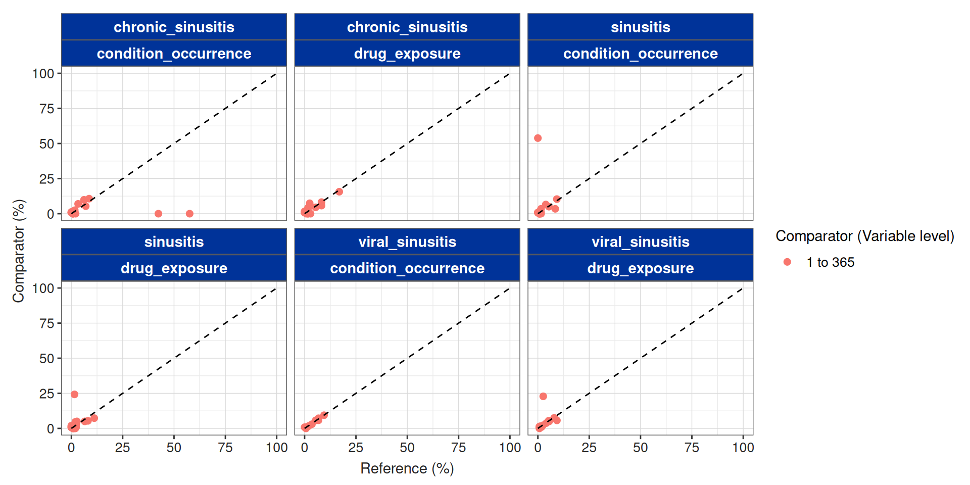
Summarise large scale characteristics

Large scale characterisation is very useful to characterise cohorts in a data driven way. You will just need to define tables and windows.

The tables need to be classified into two categories:

event: We are only interest whether the ‘start’ of the event is within the window of interest (e.g. start of the drug -> drug_exposure_start_date, start of the condition -> condition_start_date).
episode: We are interested to see whether the any day within the ‘start’ and the ‘end’ of the episode is within the window of interest.

Summarise large scale characteristics

result <- summariseLargeScaleCharacteristics(
  cohort = cdm$my_cohort,
  episodeInWindow = "drug_exposure",
  eventInWindow = "condition_occurrence",
  window = list(c(-365, -1), c(1, 365))
)

Summarise large scale characteristics

tableLargeScaleCharacteristics(
  result = result
)

Summarise large scale characteristics

tableLargeScaleCharacteristics(
  result = result,
  compareBy = "cohort_name"
)

Summarise large scale characteristics

tableLargeScaleCharacteristics(
  result = result,
  compareBy = "cohort_name",
  smdReference = "sinusitis"
)

Summarise large scale characteristics

tableLargeScaleCharacteristics(
  result = result,
  compareBy = "variable_level",
  smdReference = "-365 to -1"
)

Summarise large scale characteristics

tableTopLargeScaleCharacteristics(result = result)

	Cohort name
	chronic_sinusitis				sinusitis				viral_sinusitis
	Window
	-365 to -1		1 to 365		-365 to -1		1 to 365		-365 to -1		1 to 365
	Table name
	condition_occurrence	drug_exposure	condition_occurrence	drug_exposure	condition_occurrence	drug_exposure	condition_occurrence	drug_exposure	condition_occurrence	drug_exposure	condition_occurrence	drug_exposure
Top	Type
Top	event	episode	event	episode	event	episode	event	episode	event	episode	event	episode
1	Sinusitis (4283893) 140 (57.6%)	Amoxicillin 250 MG / Clavulanate 125 MG Oral Tablet (1713671) 41 (16.9%)	Viral sinusitis (40481087) 26 (10.7%)	Amoxicillin 250 MG / Clavulanate 125 MG Oral Tablet (1713671) 38 (15.6%)	Viral sinusitis (40481087) 24 (9.2%)	poliovirus vaccine, inactivated (40213160) 29 (11.2%)	Chronic sinusitis (257012) 140 (53.9%)	Amoxicillin 250 MG / Clavulanate 125 MG Oral Tablet (1713671) 63 (24.2%)	Viral sinusitis (40481087) 413 (9.5%)	poliovirus vaccine, inactivated (40213160) 404 (9.3%)	Viral sinusitis (40481087) 410 (9.4%)	Amoxicillin 250 MG / Clavulanate 125 MG Oral Tablet (1713671) 996 (22.8%)
2	Acute bacterial sinusitis (4294548) 103 (42.4%)	Aspirin 81 MG Oral Tablet (19059056) 20 (8.2%)	Acute viral pharyngitis (4112343) 24 (9.9%)	poliovirus vaccine, inactivated (40213160) 20 (8.2%)	Otitis media (372328) 22 (8.5%)	Aspirin 81 MG Oral Tablet (19059056) 21 (8.1%)	Viral sinusitis (40481087) 27 (10.4%)	poliovirus vaccine, inactivated (40213160) 19 (7.3%)	Acute viral pharyngitis (4112343) 295 (6.8%)	Aspirin 81 MG Oral Tablet (19059056) 346 (7.9%)	Acute viral pharyngitis (4112343) 315 (7.2%)	Aspirin 81 MG Oral Tablet (19059056) 326 (7.5%)
3	Viral sinusitis (40481087) 21 (8.6%)	poliovirus vaccine, inactivated (40213160) 20 (8.2%)	Acute bronchitis (260139) 17 (7.0%)	Acetaminophen 325 MG Oral Tablet (1127433) 18 (7.4%)	Acute viral pharyngitis (4112343) 14 (5.4%)	Acetaminophen 160 MG Oral Tablet (1127078) 17 (6.5%)	Acute bronchitis (260139) 17 (6.5%)	Aspirin 81 MG Oral Tablet (19059056) 14 (5.4%)	Otitis media (372328) 295 (6.8%)	Acetaminophen 160 MG Oral Tablet (1127078) 240 (5.5%)	Otitis media (372328) 252 (5.8%)	poliovirus vaccine, inactivated (40213160) 249 (5.7%)
4	Otitis media (372328) 17 (7.0%)	Acetaminophen 160 MG Oral Tablet (1127078) 13 (5.3%)	Otitis media (372328) 13 (5.3%)	Aspirin 81 MG Oral Tablet (19059056) 14 (5.8%)	Acute bronchitis (260139) 10 (3.9%)	Acetaminophen 325 MG Oral Tablet (1127433) 7 (2.7%)	Acute viral pharyngitis (4112343) 13 (5.0%)	Acetaminophen 160 MG Oral Tablet (1127078) 13 (5.0%)	Acute bronchitis (260139) 236 (5.4%)	Acetaminophen 325 MG Oral Tablet (1127433) 229 (5.2%)	Acute bronchitis (260139) 250 (5.7%)	Acetaminophen 325 MG Oral Tablet (1127433) 238 (5.5%)
5	Acute viral pharyngitis (4112343) 15 (6.2%)	Haemophilus influenzae type b vaccine, PRP-OMP conjugate (40213314) 7 (2.9%)	Streptococcal sore throat (28060) 6 (2.5%)	Acetaminophen 160 MG Oral Tablet (1127078) 11 (4.5%)	Fracture of ankle (4059173) 4 (1.5%)	Acetaminophen 21.7 MG/ML / Dextromethorphan Hydrobromide 1 MG/ML / doxylamine succinate 0.417 MG/ML Oral Solution (40229134) 6 (2.3%)	Otitis media (372328) 9 (3.5%)	Acetaminophen 325 MG Oral Tablet (1127433) 13 (5.0%)	Streptococcal sore throat (28060) 155 (3.6%)	Penicillin V Potassium 250 MG Oral Tablet (19133873) 180 (4.1%)	Streptococcal sore throat (28060) 131 (3.0%)	Acetaminophen 160 MG Oral Tablet (1127078) 218 (5.0%)
6	Acute bronchitis (260139) 8 (3.3%)	Acetaminophen 325 MG Oral Tablet (1127433) 6 (2.5%)	Fracture of forearm (4278672) 3 (1.2%)	Penicillin V Potassium 250 MG Oral Tablet (19133873) 10 (4.1%)	Streptococcal sore throat (28060) 4 (1.5%)	Penicillin G 375 MG/ML Injectable Solution (19006318) 6 (2.3%)	Streptococcal sore throat (28060) 9 (3.5%)	Penicillin V Potassium 250 MG Oral Tablet (19133873) 12 (4.6%)	Sprain of ankle (81151) 86 (2.0%)	Amoxicillin 250 MG / Clavulanate 125 MG Oral Tablet (1713671) 114 (2.6%)	Sprain of ankle (81151) 75 (1.7%)	Penicillin V Potassium 250 MG Oral Tablet (19133873) 166 (3.8%)
7	Whiplash injury to neck (4218389) 5 (2.1%)	Acetaminophen 21.7 MG/ML / Dextromethorphan Hydrobromide 1 MG/ML / doxylamine succinate 0.417 MG/ML Oral Solution (40229134) 4 (1.6%)	Sprain of ankle (81151) 3 (1.2%)	Penicillin G 375 MG/ML Injectable Solution (19006318) 5 (2.1%)	Whiplash injury to neck (4218389) 4 (1.5%)	Amoxicillin 250 MG Oral Capsule (19073183) 5 (1.9%)	Sprain of ankle (81151) 4 (1.5%)	Acetaminophen 21.7 MG/ML / Dextromethorphan Hydrobromide 1 MG/ML / doxylamine succinate 0.417 MG/ML Oral Solution (40229134) 7 (2.7%)	Concussion with no loss of consciousness (378001) 37 (0.8%)	Penicillin G 375 MG/ML Injectable Solution (19006318) 106 (2.4%)	Concussion with no loss of consciousness (378001) 38 (0.9%)	Penicillin G 375 MG/ML Injectable Solution (19006318) 96 (2.2%)
8	Streptococcal sore throat (28060) 4 (1.6%)	Doxycycline Monohydrate 50 MG Oral Tablet (46233988) 4 (1.6%)	Fracture of ankle (4059173) 2 (0.8%)	varicella virus vaccine (40213251) 5 (2.1%)	Concussion with no loss of consciousness (378001) 2 (0.8%)	Haemophilus influenzae type b vaccine, PRP-OMP conjugate (40213314) 5 (1.9%)	Child attention deficit disorder (440086) 2 (0.8%)	varicella virus vaccine (40213251) 5 (1.9%)	Fracture of forearm (4278672) 35 (0.8%)	Haemophilus influenzae type b vaccine, PRP-OMP conjugate (40213314) 80 (1.8%)	Acute bacterial sinusitis (4294548) 37 (0.8%)	Acetaminophen 21.7 MG/ML / Dextromethorphan Hydrobromide 1 MG/ML / doxylamine succinate 0.417 MG/ML Oral Solution (40229134) 67 (1.5%)
9	Fracture of ankle (4059173) 3 (1.2%)	Ibuprofen 100 MG Oral Tablet (19019979) 4 (1.6%)	Fracture subluxation of wrist (4134304) 2 (0.8%)	Acetaminophen 21.7 MG/ML / Dextromethorphan Hydrobromide 1 MG/ML / doxylamine succinate 0.417 MG/ML Oral Solution (40229134) 4 (1.6%)	Facial laceration (4156265) 2 (0.8%)	Penicillin V Potassium 250 MG Oral Tablet (19133873) 5 (1.9%)	First degree burn (4296204) 2 (0.8%)	{7 (Inert Ingredients 1 MG Oral Tablet) / 21 (Mestranol 0.05 MG / Norethindrone 1 MG Oral Tablet) } Pack [Norinyl 1+50 28 Day] (19128065) 4 (1.5%)	Child attention deficit disorder (440086) 34 (0.8%)	varicella virus vaccine (40213251) 65 (1.5%)	Sprain of wrist (78272) 34 (0.8%)	{7 (Inert Ingredients 1 MG Oral Tablet) / 21 (Mestranol 0.05 MG / Norethindrone 1 MG Oral Tablet) } Pack [Norinyl 1+50 28 Day] (19128065) 58 (1.3%)
10	Fracture of clavicle (4237458) 2 (0.8%)	Penicillin V Potassium 250 MG Oral Tablet (19133873) 4 (1.6%)	Laceration of hand (4113008) 2 (0.8%)	{7 (Inert Ingredients 1 MG Oral Tablet) / 21 (Mestranol 0.05 MG / Norethindrone 1 MG Oral Tablet) } Pack [Norinyl 1+50 28 Day] (19128065) 4 (1.6%)	First degree burn (4296204) 2 (0.8%)	Amoxicillin 250 MG / Clavulanate 125 MG Oral Tablet (1713671) 4 (1.5%)	Fracture of clavicle (4237458) 2 (0.8%)	Ibuprofen 100 MG Oral Tablet (19019979) 3 (1.1%)	Fracture subluxation of wrist (4134304) 29 (0.7%)	Acetaminophen 21.7 MG/ML / Dextromethorphan Hydrobromide 1 MG/ML / doxylamine succinate 0.417 MG/ML Oral Solution (40229134) 50 (1.1%)	Child attention deficit disorder (440086) 31 (0.7%)	Haemophilus influenzae type b vaccine, PRP-OMP conjugate (40213314) 46 (1.1%)

Summarise large scale characteristics

plotComparedLargeScaleCharacteristics(
  result = result,
  colour = "variable_level",
  reference = "-365 to -1",
  facet = c("cohort_name", "table_name")
)

Summarise large scale characteristics

plotComparedLargeScaleCharacteristics(
  result = result,
  colour = "variable_level",
  reference = "-365 to -1",
  facet = c("cohort_name", "table_name")
) |>
  ggplotly()

Summarise large scale characteristics

By default the large scale characterisation is run using the standard concept id (e.g. drug_concept_id), but you can also run it using a pair of standard and source concepts with the option: includeSource = TRUE.

result <- summariseLargeScaleCharacteristics(
  cohort = cdm$my_cohort,
  episodeInWindow = "drug_exposure",
  eventInWindow = "condition_occurrence",
  window = list(c(-365, -1), c(1, 365)),
  includeSource = TRUE
)

Summarise large scale characteristics

tableLargeScaleCharacteristics(result = result)

Summarise large scale characteristics

NOTE that by default any concept with a smaller frequency than 0.5% (0.005) is trimmed from the results to avoid exporting not meaningful percentages. This can be controlled by the argument minimumFrequency. Set minimumFrequency = 0 if you want to export the percentage of every single concept (suppress rules will still apply and under minCellCount counts will be removed). Also you can set a higher threshold if you are only interested in high prevalent covariates. Computationally this won’t make a difference so in general it is not recommended to change this value unless you want to set minimumFrequency = 0.

Finally, you can also exclude concepts from the search, by default the concept ID = 0 is excluded (excludedCodes = c(0)).