2Core verbs for analytic pipelines utilising a database
We saw in the previous chapter that we can use familiar dplyr verbs with data held in a database. In the last chapter we were working with just a single table which we loaded into the database. When working with databases we will though typically be working with multiple tables (as we’ll see later when working with data in the OMOP CDM format). For this chapter we will see more tidyverse functionality that can be used with data in a database, this time using the nycflights13 data. As we can see, now we have a set of related tables with data on flights departing from New York City airports in 2013.
For almost all analyses we want to go from having our starting data spread out across multiple tables in the database to a single tidy table containing all the data we need for the specific analysis. We can often get to our tidy analytic dataset using the below tidyverse functions (most of which coming from dplyr, but a couple also from the tidyr package). These functions all work with data in a database by generating SQL that will have the same purpose as if these functions were being run against data in R.
Important
Until we use compute() or collect() (or printing the first few rows of the result) all we’re doing is translating R code into SQL. Which means no code is being executed in the database side.
compute() will execute the query and store it in a new table in the database.
collect() will execute the query and bring the result back to R.
printing (e.g. glimpse() or print()) will execute the query limiting the result to the first set of rows which leads to smaller computation time in the database side.
By using the above functions we can use the same code regardless of whether the data is held in the database or locally in R. This is because the functions used above are generic functions which behave differently depending on the type of input they are given. Let’s take inner_join() for example. We can see that this function is a S3 generic function (with S3 being the most common object-oriented system used in R).
library(sloop)ftype(inner_join)
[1] "S3" "generic"
Among others, the references we create to tables in a database have tbl_lazy as a class attribute. Meanwhile, we can see that when collected into R the object changes to have different attributes, one of which being data.frame :
To see a little more on how we can use the above functions, let’s say we want to do an analysis of late flights from JFK airport. We want to see whether there is some relationship between plane characteristics and the risk of delay.
For this we’ll first use the filter() and select()dplyr verbs to get the data from the flights table. Note, we’ll rename arr_delay to just delay.
Now we’ll add plane characteristics from the planes table. We will use an inner join so that only records for which we have the plane characteristics are kept.
Note that our first query was not executed, as we didn’t use either compute() or collect(), so we’ll now have added our join to the original query.
NoteShow query
See that now the SQL code combines both queries:
<SQL>
SELECT LHS.*, seats
FROM (
  SELECT dest, distance, carrier, tailnum, arr_delay AS delay
  FROM flights
  WHERE (NOT((arr_delay IS NULL)) AND origin = 'JFK')
) LHS
INNER JOIN planes
  ON (LHS.tailnum = planes.tailnum)
And when executed, our results will look like the following:
Getting to this tidy dataset has been done in the database via R code translated to SQL. With this, we can now collect our analytic dataset into R and go from there (for example, to perform locally statistical analyses which might not be possible to run in a database such as plots, density distributions, regression, … anything beyond the data manipulation).
Now that we’ve reached the end of this example, we can close our connection to the database.
dbDisconnect(conn = con)
2.4 Further reading
Wickham H, François R, Henry L, Müller K, Vaughan D (2025). dplyr: A Grammar of Data Manipulation. R package version 1.1.4, https://dplyr.tidyverse.org
Wickham H, Vaughan D, Girlich M (2025). tidyr: Tidy Messy Data. R package version 1.3.1, https://tidyr.tidyverse.org.
Source Code
# Core verbs for analytic pipelines utilising a database {#sec-tidyverse_verbs}We saw in the previous chapter that we can use familiar [`dplyr`](https://dplyr.tidyverse.org) verbs with data held in a database. In the last chapter we were working with just a single table which we loaded into the database. When working with databases we will though typically be working with multiple tables (as we'll see later when working with data in the OMOP CDM format). For this chapter we will see more tidyverse functionality that can be used with data in a database, this time using the [`nycflights13`](https://nycflights13.tidyverse.org) data. As we can see, now we have a set of related tables with data on flights departing from New York City airports in 2013.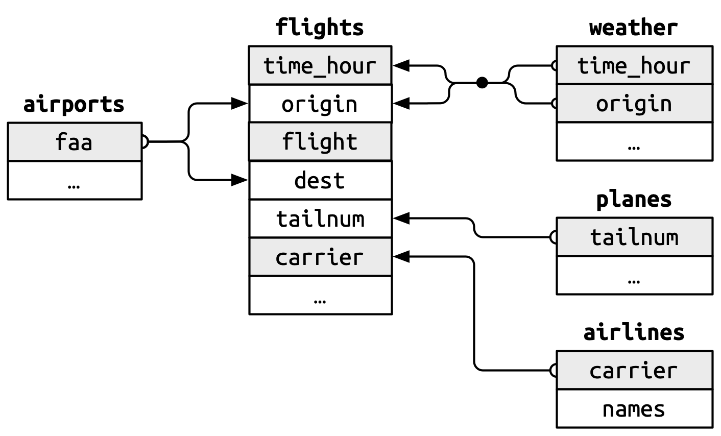{#fig-nycflights13 .lightbox}Let's load the required libraries, add our data to a DuckDB database, and then create references to each of these tables.```{r, message=FALSE, warning=FALSE}library(nycflights13)library(dplyr)library(dbplyr)library(tidyr)library(duckdb)library(DBI)# create duckdb connectioncon <-dbConnect(drv =duckdb())# copy tables in a loopfor (nm inc("airlines", "airports", "flights", "planes", "weather")) {dbWriteTable(conn = con, name = nm, value =get(nm))}airports_db <-tbl(src = con, "airports")glimpse(airports_db)flights_db <-tbl(src = con, "flights")glimpse(flights_db)weather_db <-tbl(src = con, "weather")glimpse(weather_db)planes_db <-tbl(src = con, "planes")glimpse(planes_db)airlines_db <-tbl(src = con, "airlines")glimpse(airlines_db)```## Tidyverse functionsFor almost all analyses we want to go from having our starting data spread out across multiple tables in the database to a single tidy table containing all the data we need for the specific analysis. We can often get to our tidy analytic dataset using the below tidyverse functions (most of which coming from [`dplyr`](https://dplyr.tidyverse.org), but a couple also from the [`tidyr`](https://tidyr.tidyverse.org) package). These functions all work with data in a database by generating SQL that will have the same purpose as if these functions were being run against data in R.::: callout-importantUntil we use [`compute()`](https://dplyr.tidyverse.org/reference/compute.html) or [`collect()`](https://dplyr.tidyverse.org/reference/collect.html) (or printing the first few rows of the result) all we're doing is translating R code into SQL. Which means no code is being executed in the database side.- [`compute()`](https://dplyr.tidyverse.org/reference/compute.html) will execute the query and store it in a new table in the database.- [`collect()`](https://dplyr.tidyverse.org/reference/collect.html) will execute the query and bring the result back to R.- printing (e.g. [`glimpse()`](https://pillar.r-lib.org/reference/glimpse.html) or [`print()`](https://www.rdocumentation.org/packages/base/versions/3.6.2/topics/print)) will execute the query limiting the result to the first set of rows which leads to smaller computation time in the database side.:::| Purpose | Functions | Description ||----------------|----------------------------------------|----------------|| Selecting rows |[filter](https://dplyr.tidyverse.org/reference/filter.html), [distinct](https://dplyr.tidyverse.org/reference/distinct.html)| To select rows in a table. || Ordering rows |[arrange](https://dplyr.tidyverse.org/reference/arrange.html)| To order rows in a table. || Column Transformation |[mutate](https://dplyr.tidyverse.org/reference/mutate.html), [select](https://dplyr.tidyverse.org/reference/select.html), [relocate](https://dplyr.tidyverse.org/reference/relocate.html), [rename](https://dplyr.tidyverse.org/reference/rename.html)| To create new columns or change existing ones. || Grouping and ungrouping |[group_by](https://dplyr.tidyverse.org/reference/group_by.html), [rowwise](https://dplyr.tidyverse.org/reference/rowwise.html), [ungroup](https://dplyr.tidyverse.org/reference/ungroup.html)| To group data by one or more variables and to remove grouping. || Aggregation |[count](https://dplyr.tidyverse.org/reference/count.html), [tally](https://dplyr.tidyverse.org/reference/tally.html), [summarise](https://dplyr.tidyverse.org/reference/summarise.html)| These functions are used for summarising data. || Data merging and joining |[inner_join](https://dplyr.tidyverse.org/reference/mutate-joins.html), [left_join](https://dplyr.tidyverse.org/reference/mutate-joins.html), [right_join](https://dplyr.tidyverse.org/reference/mutate-joins.html), [full_join](https://dplyr.tidyverse.org/reference/mutate-joins.html), [anti_join](https://dplyr.tidyverse.org/reference/filter-joins.html), [semi_join](https://dplyr.tidyverse.org/reference/filter-joins.html), [cross_join](https://dplyr.tidyverse.org/reference/cross_join.html)| These functions are used to combine data from different tables based on common columns. || Data reshaping |[pivot_wider](https://tidyr.tidyverse.org/reference/pivot_wider.html), [pivot_longer](https://tidyr.tidyverse.org/reference/pivot_longer.html)| These functions are used to reshape data between wide and long formats. || Data union |[union_all](https://dplyr.tidyverse.org/reference/setops.html), [union](https://dplyr.tidyverse.org/reference/setops.html)| This function combines two tables. || Randomly selects rows |[slice_sample](https://dplyr.tidyverse.org/reference/slice.html)| We can use this to take a random subset a table. |::: {.callout-tip collapse="true"}### Behind the scenesBy using the above functions we can use the same code regardless of whether the data is held in the database or locally in R. This is because the functions used above are generic functions which behave differently depending on the type of input they are given. Let's take [`inner_join()`](https://dplyr.tidyverse.org/reference/mutate-joins.html) for example. We can see that this function is a S3 generic function (with S3 being the most common object-oriented system used in R).```{r, message=FALSE, warning=FALSE}library(sloop)ftype(inner_join)```Among others, the references we create to tables in a database have `tbl_lazy` as a class attribute. Meanwhile, we can see that when collected into R the object changes to have different attributes, one of which being `data.frame` :```{r, message=FALSE, warning=FALSE}class(flights_db)class(flights_db |>head(1) |>collect())```We can see that [`inner_join()`](https://dplyr.tidyverse.org/reference/mutate-joins.html) has different methods for `tbl_lazy` and `data.frame`.```{r, message=FALSE, warning=FALSE}s3_methods_generic("inner_join")```When working with references to tables in the database the `tbl_lazy` method will be used.```{r, message=FALSE, warning=FALSE}s3_dispatch(flights_db |>inner_join(planes_db))```But once we bring data into R, the `data.frame` method will be used.```{r, message=FALSE, warning=FALSE}s3_dispatch(flights_db |>head(1) |>collect() |>inner_join(planes_db |>head(1) |>collect()))```:::## Getting to an analytic datasetTo see a little more on how we can use the above functions, let's say we want to do an analysis of late flights from JFK airport. We want to see whether there is some relationship between plane characteristics and the risk of delay.For this we'll first use the [`filter()`](https://dplyr.tidyverse.org/reference/filter.html) and [`select()`](https://dplyr.tidyverse.org/reference/filter.html)[`dplyr`](https://dplyr.tidyverse.org) verbs to get the data from the flights table. Note, we'll rename arr_delay to just delay.```{r, message=FALSE, warning=FALSE}delayed_flights_db <- flights_db |>filter(!is.na(arr_delay) & origin =="JFK") |>select("dest", "distance", "carrier", "tailnum", "delay"="arr_delay")```::: {.callout-note collapse="true"}### Show querySee the resultant DuckDB query:```{r, message=FALSE, warning=FALSE, echo=FALSE}show_query(delayed_flights_db)```:::When executed, our results will look like the following:```{r, message=FALSE, warning=FALSE}delayed_flights_db```Now we'll add plane characteristics from the planes table. We will use an inner join so that only records for which we have the plane characteristics are kept.```{r, message=FALSE, warning=FALSE}delayed_flights_db <- delayed_flights_db |>inner_join( planes_db |>select("tailnum", "seats"),by ="tailnum" )```Note that our first query was not executed, as we didn't use either [`compute()`](https://dplyr.tidyverse.org/reference/compute.html) or [`collect()`](https://dplyr.tidyverse.org/reference/collect.html), so we'll now have added our join to the original query.::: {.callout-note collapse="true"}### Show querySee that now the SQL code combines both queries:```{r, message=FALSE, warning=FALSE, echo=FALSE}show_query(delayed_flights_db)```:::And when executed, our results will look like the following:```{r, message=FALSE, warning=FALSE}delayed_flights_db```Getting to this tidy dataset has been done in the database via R code translated to SQL. With this, we can now collect our analytic dataset into R and go from there (for example, to perform locally statistical analyses which might not be possible to run in a database such as plots, density distributions, regression, ... anything beyond the data manipulation).```{r, message=FALSE, warning=FALSE}delayed_flights <- delayed_flights_db |>collect() glimpse(delayed_flights)```## Disconnecting from the databaseNow that we've reached the end of this example, we can close our connection to the database.```{r}dbDisconnect(conn = con)```## Further reading- Wickham H, François R, Henry L, Müller K, Vaughan D (2025). *dplyr: A Grammar of Data Manipulation*. R package version 1.1.4, <https://dplyr.tidyverse.org>- Wickham H, Vaughan D, Girlich M (2025). *tidyr: Tidy Messy Data*. R package version 1.3.1, <https://tidyr.tidyverse.org>.
