library(DBI)
library(dbplyr)
library(dplyr)
library(here)
library(CDMConnector)
library(ggplot2)
library(clock)6 Exploring the OMOP CDM
For this chapter, we’ll use a synthetic Covid-19 dataset.
db<-dbConnect(duckdb::duckdb(),
              dbdir = eunomiaDir(datasetName = "synthea-covid19-10k"))
cdm <- cdmFromCon(db, cdmSchema = "main", writeSchema = "main")cdm── # OMOP CDM reference (duckdb) of Synthea ────────────────────────────────────• omop tables: attribute_definition, care_site, cdm_source, cohort_definition,
concept, concept_ancestor, concept_class, concept_relationship,
concept_synonym, condition_era, condition_occurrence, cost, death,
device_exposure, domain, dose_era, drug_era, drug_exposure, drug_strength,
fact_relationship, location, measurement, metadata, note, note_nlp,
observation, observation_period, payer_plan_period, person,
procedure_occurrence, provider, relationship, source_to_concept_map, specimen,
visit_detail, visit_occurrence, vocabulary• cohort tables: -• achilles tables: -• other tables: -6.1 Counting people
The OMOP CDM is person-centric, with the person table containing records to uniquely identify each person in the database. As each row refers to a unique person, we can quickly get a count of the number of individuals in the database like so
cdm$person |>
  count()
# Source: SQL [?? x 1]
# Database: DuckDB 1.3.3-dev231 [unknown@Linux 6.11.0-1018-azure:R 4.4.1//tmp/RtmprL7faW/file2e322f8f86ff.duckdb]
n
<dbl>
1 10754The person table also contains some demographic information, including a gender concept for each person. We can get a count grouped by this variable, but as this uses a concept we’ll also need to join to the concept table to get the corresponding concept name for each concept id.
cdm$person |>
  group_by(gender_concept_id) |>
  count() |>
  left_join(cdm$concept,
            by=c("gender_concept_id" = "concept_id")) |>
              select("gender_concept_id", "concept_name", "n") |>
  collect()
# A tibble: 2 × 3
# Groups: gender_concept_id [2]
gender_concept_id concept_name n
<int> <chr> <dbl>
1 8532 FEMALE 5165
2 8507 MALE 5589
Vocabulary tables
Above we’ve got counts by specific concept IDs recorded in the condition occurrence table. What these IDs represent is described in the concept table. Here we have the name associated with the concept, along with other information such as it’s domain and vocabulary id.
cdm$concept |>
  glimpse()
Rows: ??
Columns: 10
Database: DuckDB 1.3.3-dev231 [unknown@Linux 6.11.0-1018-azure:R 4.4.1//tmp/RtmprL7faW/file2e322f8f86ff.duckdb]
$ concept_id <int> 45756805, 45756804, 45756803, 45756802, 45756801, 457…
$ concept_name <chr> "Pediatric Cardiology", "Pediatric Anesthesiology", "…
$ domain_id <chr> "Provider", "Provider", "Provider", "Provider", "Prov…
$ vocabulary_id <chr> "ABMS", "ABMS", "ABMS", "ABMS", "ABMS", "ABMS", "ABMS…
$ concept_class_id <chr> "Physician Specialty", "Physician Specialty", "Physic…
$ standard_concept <chr> "S", "S", "S", "S", "S", "S", "S", "S", "S", "S", "S"…
$ concept_code <chr> "OMOP4821938", "OMOP4821939", "OMOP4821940", "OMOP482…
$ valid_start_date <date> 1970-01-01, 1970-01-01, 1970-01-01, 1970-01-01, 1970…
$ valid_end_date <date> 2099-12-31, 2099-12-31, 2099-12-31, 2099-12-31, 2099…
$ invalid_reason <chr> NA, NA, NA, NA, NA, NA, NA, NA, NA, NA, NA, NA, NA, N…Other vocabulary tables capture other information about concepts, such as the direct relationships between concepts (the concept relationship table) and hierarchical relationships between (the concept ancestor table).
cdm$concept_relationship |>
  glimpse()
Rows: ??
Columns: 6
Database: DuckDB 1.3.3-dev231 [unknown@Linux 6.11.0-1018-azure:R 4.4.1//tmp/RtmprL7faW/file2e322f8f86ff.duckdb]
$ concept_id_1 <int> 35804314, 35804314, 35804314, 35804327, 35804327, 358…
$ concept_id_2 <int> 912065, 42542145, 42542145, 35803584, 42542145, 42542…
$ relationship_id <chr> "Has modality", "Has accepted use", "Is current in", …
$ valid_start_date <date> 2021-01-26, 2019-08-29, 2019-08-29, 2019-05-27, 2019…
$ valid_end_date <date> 2099-12-31, 2099-12-31, 2099-12-31, 2099-12-31, 2099…
$ invalid_reason <chr> NA, NA, NA, NA, NA, NA, NA, NA, NA, NA, NA, NA, NA, N…cdm$concept_ancestor |>
glimpse()Rows: ??
Columns: 4
Database: DuckDB 1.3.3-dev231 [unknown@Linux 6.11.0-1018-azure:R 4.4.1//tmp/RtmprL7faW/file2e322f8f86ff.duckdb]
$ ancestor_concept_id <int> 375415, 727760, 735979, 438112, 529411, 14196…
$ descendant_concept_id <int> 4335743, 2056453, 41070383, 36566114, 4326940…
$ min_levels_of_separation <int> 4, 1, 3, 2, 3, 3, 4, 3, 2, 5, 1, 3, 4, 2, 2, …
$ max_levels_of_separation <int> 4, 1, 5, 3, 3, 6, 12, 3, 2, 10, 1, 3, 4, 2, 2…More information on the vocabulary tables (as well as other tables in the OMOP CDM version 5.3) can be found at https://ohdsi.github.io/CommonDataModel/cdm53.html#Vocabulary_Tables.
6.2 Summarising observation periods
The observation period table contains records indicating spans of time over which clinical events can be reliably observed for the people in the person table. Someone can potentially have multiple observation periods. So say we wanted a count of people grouped by the year during which their first observation period started. We could do this like so:
first_observation_period <- cdm$observation_period |>
    group_by(person_id) |>
    filter(row_number() == 1) |>
    compute()

cdm$person |>
  left_join(first_observation_period,
            by = "person_id") |>
  mutate(observation_period_start_year = get_year(observation_period_start_date)) |>
  group_by(observation_period_start_year) |>
  count() |>
  collect() |>
  ggplot() +
  geom_col(aes(observation_period_start_year, n)) +
  theme_bw()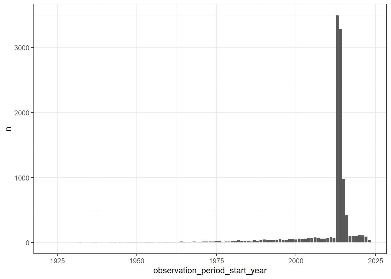
6.3 Summarising clinical records
What’s the number of condition occurrence records per person in the database? We can find this out like so
cdm$person |>
  left_join(cdm$condition_occurrence |>
  group_by(person_id) |>
  count(name = "condition_occurrence_records"),
  by="person_id") |>
  mutate(condition_occurrence_records = if_else(
    is.na(condition_occurrence_records), 0,
    condition_occurrence_records)) |>
  group_by(condition_occurrence_records) |>
  count() |>
  collect() |>
  ggplot() +
  geom_col(aes(condition_occurrence_records, n)) +
  theme_bw()
How about we were interested in getting record counts for some specific concepts related to Covid-19 symptoms?
cdm$condition_occurrence |>
  filter(condition_concept_id %in% c(437663,437390,31967,
                                     4289517,4223659, 312437,
                                     434490,254761,77074)) |>
  group_by(condition_concept_id) |>
  count() |>
  left_join(cdm$concept,
            by=c("condition_concept_id" = "concept_id")) |>
  collect() |>
  ggplot() +
  geom_col(aes(concept_name, n)) +
  theme_bw()+
  xlab("")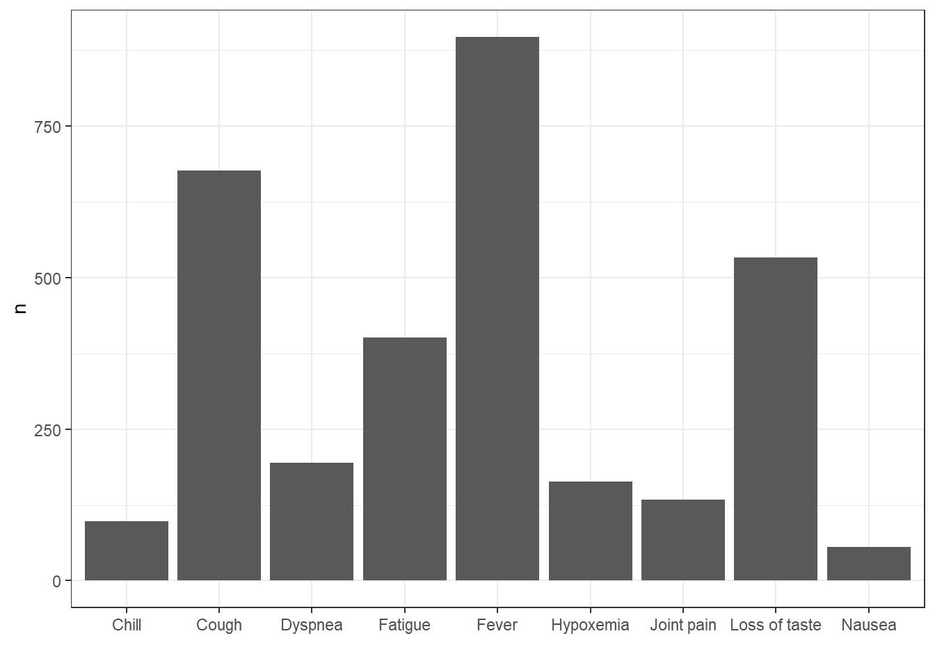
We can also use summarise for various other calculations
cdm$person |>
  summarise(min_year_of_birth = min(year_of_birth, na.rm=TRUE),
            q05_year_of_birth = quantile(year_of_birth, 0.05, na.rm=TRUE),
            mean_year_of_birth = round(mean(year_of_birth, na.rm=TRUE),0),
            median_year_of_birth = median(year_of_birth, na.rm=TRUE),
            q95_year_of_birth = quantile(year_of_birth, 0.95, na.rm=TRUE),
            max_year_of_birth = max(year_of_birth, na.rm=TRUE)) |>
  glimpse()
Rows: ??
Columns: 6
Database: DuckDB 1.3.3-dev231 [unknown@Linux 6.11.0-1018-azure:R 4.4.1//tmp/RtmprL7faW/file2e322f8f86ff.duckdb]
$ min_year_of_birth <int> 1923
$ q05_year_of_birth <dbl> 1927
$ mean_year_of_birth <dbl> 1971
$ median_year_of_birth <dbl> 1970
$ q95_year_of_birth <dbl> 2018
$ max_year_of_birth <int> 2023As we’ve seen before, we can also quickly get results for various groupings or restrictions
grouped_summary <- cdm$person |>
   group_by(gender_concept_id) |>
   summarise(min_year_of_birth = min(year_of_birth, na.rm=TRUE),
            q25_year_of_birth = quantile(year_of_birth, 0.25, na.rm=TRUE),
            median_year_of_birth = median(year_of_birth, na.rm=TRUE),
            q75_year_of_birth = quantile(year_of_birth, 0.75, na.rm=TRUE),
            max_year_of_birth = max(year_of_birth, na.rm=TRUE)) |>
  left_join(cdm$concept,
            by=c("gender_concept_id" = "concept_id")) |>
   collect()

grouped_summary |>
  ggplot(aes(x = concept_name, group = concept_name,
             fill = concept_name)) +
  geom_boxplot(aes(
    lower = q25_year_of_birth,
    upper = q75_year_of_birth,
    middle = median_year_of_birth,
    ymin = min_year_of_birth,
    ymax = max_year_of_birth),
    stat = "identity", width = 0.5) +
  theme_bw()+
  theme(legend.position = "none") +
  xlab("")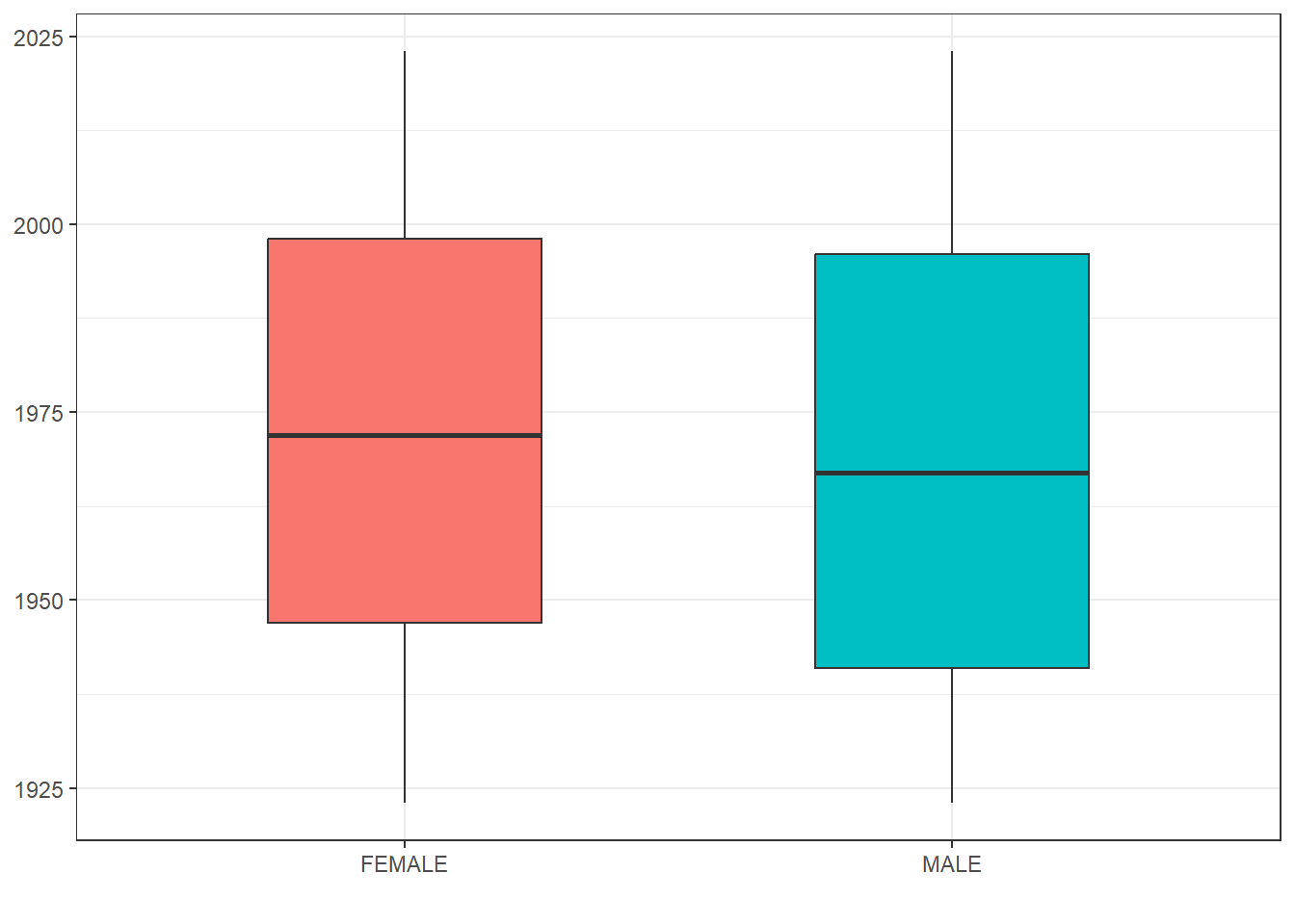
What’s the number of condition occurrence records per person in the database? We can find this out like so
cdm$person |>
  left_join(cdm$condition_occurrence |>
  group_by(person_id) |>
  count(name = "condition_occurrence_records"),
  by="person_id") |>
  mutate(condition_occurrence_records = if_else(
    is.na(condition_occurrence_records), 0,
    condition_occurrence_records)) |>
  group_by(condition_occurrence_records) |>
  count() |>
  collect() |>
  ggplot() +
  geom_col(aes(condition_occurrence_records, n)) +
  theme_bw()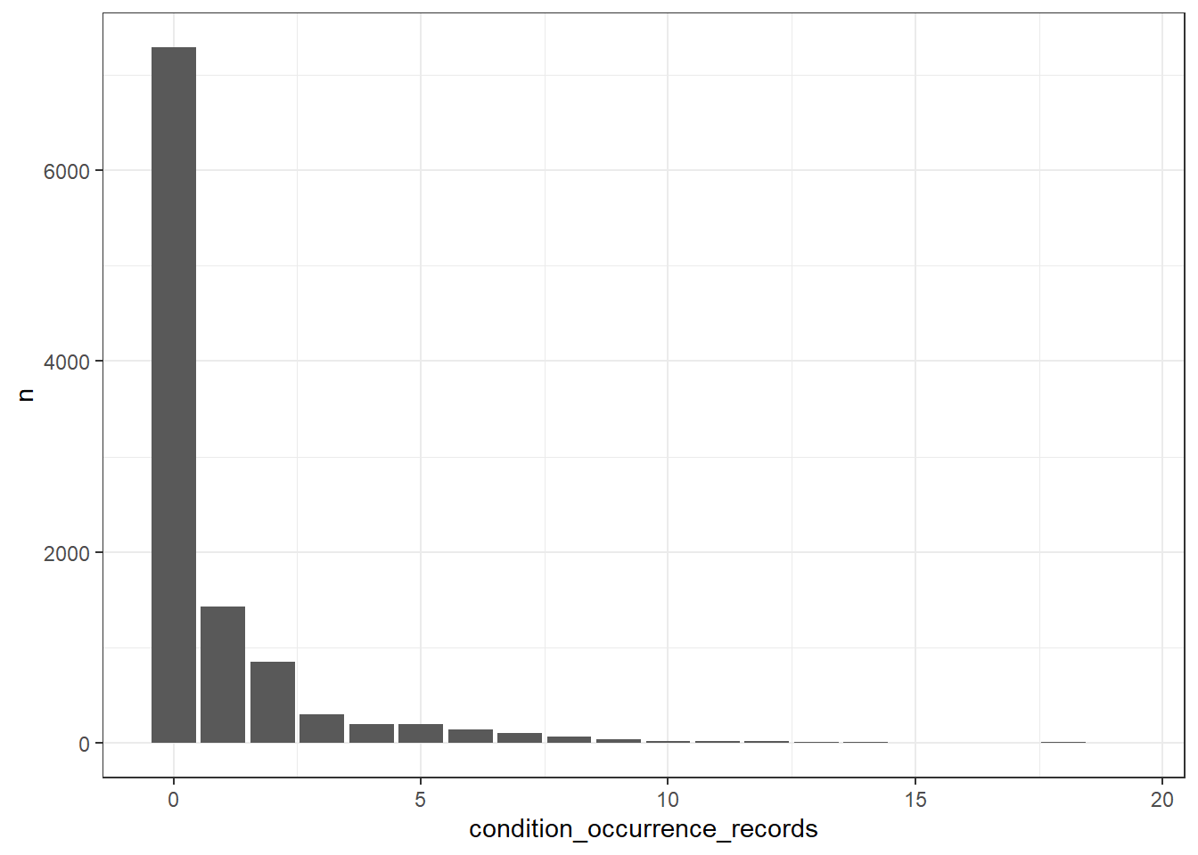
How about we were interested in getting record counts for some specific concepts related to Covid-19 symptoms?
cdm$condition_occurrence |>
  filter(condition_concept_id %in% c(437663,437390,31967,
                                     4289517,4223659, 312437,
                                     434490,254761,77074)) |>
  group_by(condition_concept_id) |>
  count() |>
  left_join(cdm$concept,
            by=c("condition_concept_id" = "concept_id")) |>
  collect() |>
  ggplot() +
  geom_col(aes(concept_name, n)) +
  theme_bw()+
  xlab("")